Unlock the conditional expectation

An motivating example

Suppose you have a wooden rod of a random length $L$, say uniformly distributed on $(0,1)$ (in meter). Then you will cut this rod a some point $X\in(0,L)$. Our question is what is the average of $X$? Given $L=\ell$ , you would say that $\mathbf{E}(X)=\frac{\ell}{2}$, isn’t it? It is true to think about it in this way. However, this answer depends on the prior knowledge of $L=\ell$ while we need  $\mathbf{E}(X)$ to equal a constant number at the end. Here where conditional expectation pops up, we can say that : the conditional expectation of $X$ given $L$ is $L/2$.

I took this example from the wonderful lectures of Prof. Joe Blitzstein. 

Conditional expectation

Definition 1. If $X$ and $Y$ are two random variables, then the conditional probability distribution function of $X$, given that $Y=y$, is defined for all $y$ such that $\mathbf{P}(Y=y)>0$, by $$p_{X\mid Y}(x\mid y)=\frac{p_{X,Y}(x,y)}{p_{Y}(y)}.$$

It is therefore natural to define, in this case, the conditional expectation of $X$ given that $Y=y$, for all values of $y$ such that $p_{Y}(y)>0$, by $$\mathbf{E}(X\mid Y=y)=\int x p_{X\mid Y}(x\mid y).$$

Note that this definition should be understood in both discrete and continuous settings. 

Definition 2. The conditional expectation of $X$ given $Y$ is the function $\mathbf{E}(X\mid Y=y)$ evaluated at $y=Y$. We denote such an expectation by $$\mathbf{E}(X\mid Y).$$

Please remember : 

⚠️ Do not substitute before computing !!!

⚠️ The conditional expectation is a random variable in terms of the variable you are conditioning on.

The conditional expectation has the following core properties :

1. $\mathbf{E}(X\mid Y)$ behaves like the ordinary expectation w.r.t the first input (linearity, positivity etc …).

2. $\mathbf{E}(Xg(Y)\mid Y)=g(Y)\mathbf{E}(X\mid Y)$. We refer to this as “Taking Out What Is Known”.

3. $\mathbf{E}(\mathbf{E}(X\mid Y))=\mathbf{E}(X)$. We refer to this as “Adam’s law” or “Law of Total Expectation”.

4. $\mathbf{E}(g(Y)\mid Y)=g(Y)$. We refer to this as “Measurability property”. 

5. $\mathbf{E}(X\mid Y)=\mathbf{E}(X)$ as long as $X$ and $Y$ are independent. Personally, I refer to this as “Blind Conditioning”.

In our introductory example, we have $\mathbf{E}(X \mid L) = \frac{L}{2}.$ Then, by the law of total expectation, it follows that $$\mathbf{E}(X) = \mathbf{E}\left(\frac{L}{2}\right) = \frac{1}{4}.$$

Applications of conditional expectation

Using conditional expectation, we can define also the conditional variance by : $$\mathbf{Var}(X\mid Y)=\mathbf{E}((X-\mathbf{E}(X\mid Y))^{2})=\mathbf{E}(X^{2}\mid Y)-\mathbf{E}(X\mid Y)^{2}.$$

In particular, on has the following result, referred to as “variance decomposition formula” : $$\mathbf{Var}(X)=\mathbf{E}(\mathbf{Var}(X\mid Y))=\mathbf{E}(X^{2}\mid Y)-\mathbf{Var}(\mathbf{E}(X\mid Y)).$$

The conditional expectation $\mathbb{E  }(X \mid Y)$ is the best predictor of $X$ given $Y$ in the sense of least squares. It is characterized by the orthogonality principle, which states that the prediction error $X – \mathbb{E}(X \mid Y)$ is uncorrelated with any function of $Y$. In other words, for any function $g(Y)$,
\[
\mathbb{E}\left[\big(X – \mathbb{E}(X \mid Y)\big) \cdot g(Y)\right] = 0.
\]
This orthogonality condition implies that $\mathbb{E}(X \mid Y)$ is the unique element in the space of $Y$-measurable functions that is closest to $X$ in $L^2$ norm. It minimizes the mean squared error among all functions of $Y$:
\[
\mathbb{E}(X \mid Y) = \arg\min_{g(Y)} \mathbb{E}\left[(X – g(Y))^2\right].
\]

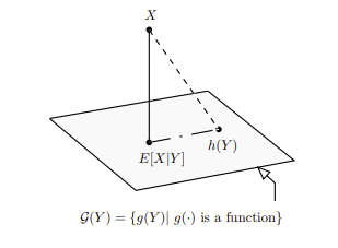
Illustration of the idea of orthogonal projection of the conditional expectation

(photo taken from Probability in Electrical Engineering and Computer Science)

This optimality makes it fundamental in fields such as regression, filtering, and stochastic control, where predicting unknown quantities based on partial information is essential.

Conclusion