On randomness

According to Oxford Dictionary, the word “Randomness” refers to the apparent or actual lack of definite pattern or predictability in information.\pause\ That is, most phenomena in life are random. For example :

• Weather condition.

• Gold price.

• Reaction of your wife after giving her a gift. 

• etc …

Definition 1. A random experiment is a procedure with the following three features : 

• A known set of outcomes $\Omega$ . $\Omega$ is called sample space. 

• Uncertainty: Unpredictable outcome when running the experiment. 

• Can be repeated infinitely many time in an independent way. Every time one performs the experiment, it is like you are performing it for the first time.

Let $E$ be some random experiment of sample space $\Omega$. An event is a set formed by some outcomes of the experiment. That is an event is a subset of $\Omega$ . 

Definition 2. A system of events $\mathscr{F}$ is called $\sigma$-algebra if :

• $\Omega\in\mathscr{F}$.

• $\mathscr{F}$ is stable under the complement operation.

• $\mathscr{F}$ is stable under countable union.

Definition 3. A probability measure is a function $\mathbf{P}$ acting on $\mathscr{F}$ and landing on the interval $[0,1]$, subject to the following rules :

• $\mathbf{P}(\emptyset)=0$.

• $\mathbf{P}(\sum A_{n})=\sum\mathbf{P}(A_{n})$, where $\Sigma$ means the events $A_{n}$ are pairwise disjoint. 

The ordered triple $(\Omega,\mathscr{F},\mathbf{P})$ is hence called a “probabilistic model” (of the underlying experiment) or a “probability space”.

Examples

Typical examples of $\sigma$-algebra are the Borel $\sigma$-algebra, the power set of $\Omega$ when it is countable etc … Here are some examples of probability spaces. 

• Uniform probability space on a finite set of outcomes $\Omega$ . The probabilistic model is simply $(\Omega,2^{\Omega},\mathbf{P})$ with $\mathbf{P}$ is defined for any $A\in2^{\Omega}$ by $$\mathbf{P}(A)=\frac{\text{card}(A)}{\text{card}(\Omega)}$$. Such a model can not be carried out by an infinite set $\Omega$ . 

• Let $f$ be some non negative nice function defined on some interval I. The triple $(I,\mathcal{B}(I),\mathbf{P})$, where $\mathbf{P}$ is defined by $$\mathbf{P}(A)=\int_{A}f(x)dx$$ for any $A\in\mathcal{B}(I)$, is a probability space. 

Random variables

In practice, people make decisions upon random experiments. For example, based on the daily Gold price, sellers adjust the prices of their goods.

Definition 6. A random variable $\xi$ is a measurable function acting on a probability space $(\Omega,\mathscr{F},\mathbf{P})$ and taking values on some $\sigma$-algebra $(R,\mathscr{R})$. That is, for any $S\in\mathscr{R}$, we have $\xi^{-1}(S)\in\mathscr{F}$.The support of $\xi$ is $\xi(\Omega)$ : the values generated by $\xi$.

In this context, one can think of a random variable as the action/decision taken based on some random experiment.

Definition 7. The law/probability distribution of $\xi$ is simply the push-forward measure of $\mathbf{P}$, say $\mathbf{P}_{\xi}$, which is defined on $\mathscr{R}$ by $$\mathbf{P}_{\xi}(S):=\mathbf{P}(\xi^{-1}(S))$$ with $S\in\mathscr{R}$. Recall that $\xi^{-1}(S)=\{\omega\in\Omega\mid\xi(\omega)\in S\}$.

We say that two random variables $\xi$ and $\Lambda$ are equal in distribution if they both have the same law. 

Relevant statistical quantities

Definition 8. The cumulative distribution function of a random variable $\xi$ is the function $$F_{\xi}:x\in\mathbb{R}\longmapsto\mathbf{P}_{\xi}((-\infty,x])=\mathbf{P}(\{\xi\leq x\}).$$

• $\xi$ is called discrete if \xi(\Omega) is countable.

• $\xi$ is called continuous if $$F_{\xi}(x)=\int_{-\infty}^{x}f(t)dt$$ for some non-negative function $f$.

The cumulative distribution function has the following properties :

• $F_{\xi}$ is non decreasing.\pause

• $F_{\xi}(-\infty)=0$.

• $F_{\xi}(+\infty)=1$.

• $F_{\xi}$ is càd-làg : continuous from the left, bounded from the right. 

• $\mathbf{P}_{\xi}(\{x\})=F_{\xi}(x)-F_{\xi}(x^{-})$.

When $\xi$ is discrete, $\xi(\Omega)=\{x_{i}\}_{i}$, then the family $\{p_{i}=\mathbf{P}_{\xi}(\{x_{i}\})\}_{i}$ is called the probability mass function of $\xi$ . We write $$dF_{\xi}(x)=\sum p_{i}\delta_{x_{i}}.$$

When $\xi$ is continuous, then the function $f$ (mentioned above) is called the probability density function of $\xi$ . We write $$dF_{\xi}=f(x)dx.$$

Definition 9. The expected value of $\xi$ is defined by $${\displaystyle \mathbf{E}(\xi)=\int xdF_{\xi}(x)=\begin{cases}
{\displaystyle \sum x_{i}p_{i}} & \text{(discrete)}\\
{\displaystyle \int xf(x)dx} & \text{(continuous)}
\end{cases}}$$ provided that $\int\vert x\vert dF_{\xi}(x)$ is finite.  Likewise, if $g$ is a measurable function, we define $$\mathbf{E}(g(\xi))=\int g(x)dF_{\xi}(x)=\begin{cases}
{\displaystyle \sum g(x_{i})p_{i}}\\
{\displaystyle \int g(x)f(x)dx}
\end{cases}.$$

Common names for expectation are expected value, mean, average.

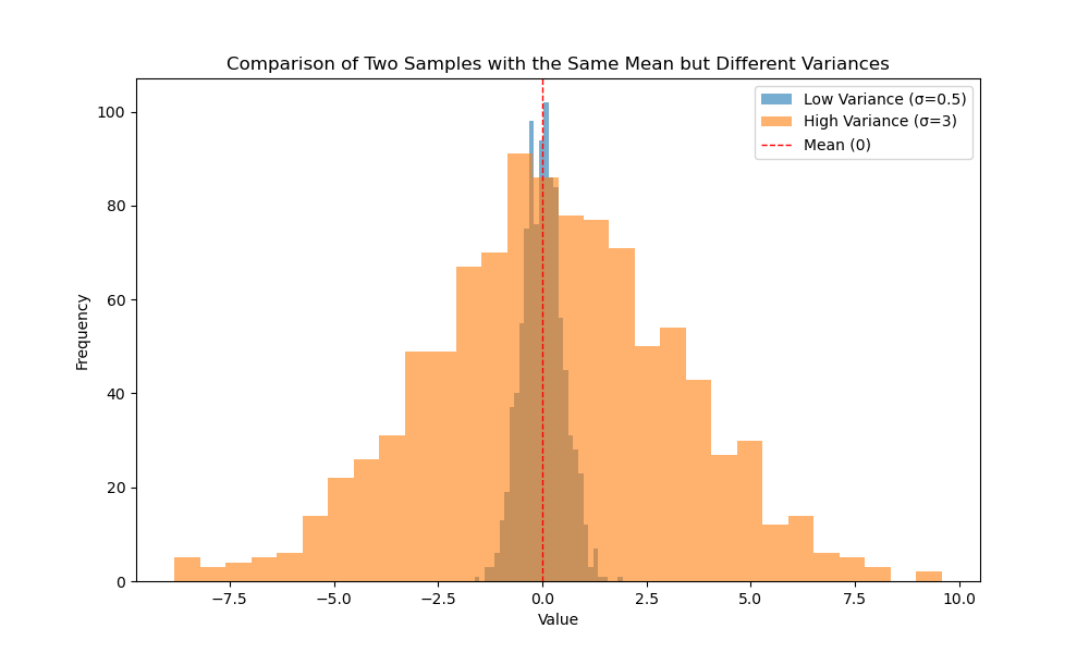
Definition 10. The variance of $\xi$ is $$\mathbf{V}(\xi)=\mathbf{E}((\xi-\mathbf{E}(\xi))^{2})=\mathbf{E}(\xi^{2})-\mathbf{E}(\xi)^{2}.$$

In particular, $\mathbf{V}(\xi)\geq0$ and $\mathbf{V}(\xi)=0$ if and only if $\xi=\mathbf{E}(\xi)$. The standard deviation of $\xi$ is $\mathbf{SD}(\xi)=\sqrt{\mathbf{Var}(\xi)}$.

Note that the expectation is a linear operator. The variance operator is not linear, rather it is quadratic. The genuine meaning of the expected value is the following : $\mathbf{E}(\xi)$ is the closest constant to $\xi$ using the quadratic integration distance. In other words, $$ \mathbf{E}(\xi)=\arg\min_{a\in\mathbb{R}}\mathbf{E}((\xi-a)^{2}) $$

🚨 ⚠️ The average, or mean, is often used as a simple summary of data, but it can be misleading without considering the underlying variability. While the mean provides a single value representing the central tendency, it doesn’t account for the spread or dispersion of the data, which can significantly influence the interpretation. For example, if most of the data points are clustered around a certain value, but a few extreme outliers exist, the mean may give a skewed representation of the typical case. In such situations, additional measures like variance or standard deviation are crucial for understanding the true nature of the data.

Consider two scenarios involving ten people: In the first, one person owns 10 million dinars, while the others have nothing. n the second, each person has 1 million dinars.

In both cases, the average wealth per individual is 1 million dinars. However, it’s clear that in the first scenario, the community is essentially poor, despite the average suggesting otherwise.