Taming the Beast: Conquer Differential Calculus with Confidence (Part two)

In our first discussion on differential calculus, we introduced the notion of differentiability for a multivariate function \( f \). In this note, we explore the concept in greater depth. Let $$ f(x_1, \dots, x_n) = f(\mathbf{x}) $$ be a real-valued function defined on some open subset \( U \subset \mathbb{R}^n .

Definition. The partial derivatives of \( f \) are simply the directional derivatives in the directions of the canonical basis vectors of \( \mathbb{R}^n \). For each \( i = 1, \dots, n \), we define:
\[
\frac{\partial f}{\partial x_i}(\mathbf{x}) = \partial_i f(\mathbf{x}) = D_{e_i}(f)(\mathbf{x}) = \lim_{t \to 0} \frac{f(x_1, \dots, x_i + t, \dots, x_n) – f(x_1, \dots, x_n)}{t}.
\]
These are evaluated at a point \( \mathbf{x} = (x_1, \dots, x_n) \in U \).

If \( f \) is differentiable at \( \mathbf{x} \), then all the partial derivatives exist at \( \mathbf{x} \), and moreover,
\[
\frac{\partial f}{\partial x_i}(\mathbf{x}) = df_{\mathbf{x}}(e_i).
\]

Partial derivatives do not even imply continuity !!! 

However, the converse is false. That is, the existence of partial derivatives does not in general imply differentiability. In fact, partial derivatives may exist without even guaranteeing continuity of the function! Consider the classical example:
\[
f(x, y) =
\begin{cases}
\frac{xy}{x^2 + y^2} & \text{if } (x, y) \neq (0, 0), \\
0 & \text{if } (x, y) = (0, 0).
\end{cases}
\]
This function admits partial derivatives at the origin, but is not continuous there. The explanation is because lines are a very limited category of paths to approach a point. 

Nevertheless, if the partial derivatives \( \partial_i f \) exist and are continuous in a neighborhood of a point, then \( f \) is differentiable at that point. More generally:

Theorem. $df_{\mathbf{x}}$ is continuous if and only if the $\partial_{i}f$’s are continuous.

A function \( f \) is said to be of class \( \mathcal{C}^1 \) if its differential \( df_{\mathbf{x}} \) is continuous for all \( \mathbf{x} \in U \), which is equivalent to saying that all its partial derivatives exist and are continuous on \( U \).

Differential of a composition

Assume we have two functions \( f \) and \( g \), and let \( h = g \circ f \). Don’t worry about domains for now — the question is: what is the differential of \( h \)? Let’s build the answer step by step:

\[
\begin{alignedat}{1}
h(x + h) &= g(f(x + h)) \\
&= g\left(f(x) + \underbrace{df_{x}(h) + \epsilon(h)}_{\widetilde{h}}\right) \\
&= g(f(x)) + dg_{f(x)}(\widetilde{h}) + \varepsilon(\widetilde{h}) \\
&= g(f(x)) + dg_{f(x)}(df_{x}(h)) + dg_{f(x)}(\epsilon(h)) + \varepsilon(\widetilde{h}) \\
&= h(x) + (dg_{f(x)} \circ df_{x})(h) + o(h)
\end{alignedat}
\]

So, we see that
\[
dh_{x} = dg_{f(x)} \circ df_{x}.
\]

At this point, you might be asking: why is \( dg_{f(x)}(\epsilon(h)) + \varepsilon(\widetilde{h}) \) an \( o(h) \) term? Well, thanks to the continuity of the linear maps \( dg_{f(x)} \) and \( df_{x} \), and the fact that \( \epsilon(h) \to 0 \) faster than \( h \), we can show that this remainder is indeed of smaller order than \( h \) as \( h \to 0 \).

Matrix representation 

As differentials are linear maps, then it is natural to represent them by matrices. That is, if $f=f_1,…,f_p)$ (the $f_i$ are the components of $f$) then the matrix of $f$ is called the Jacobian matrix of $f$ and it is equal to 

$$ J_\mathbf{x}(f):=\left[\frac{\partial f_{i}}{\partial x_{i}}(\mathbf{x})\right]_{i,j}$$

In particular, if $h$ is a vector (row represented) then 

$$df_{\mathbf{x}}(h)=J_{\mathbf{x}}(f)h^{T}$$

You may reformulate the differential of the composition now as : 

$$J_\mathbf{x}(g\circ f)=J_{f(\mathbf{x})}(g)J_\mathbf{x}(f) $$

A particular case : the Gradient 

When $f$ is real valued then it s Jacobian matrix is called Gradient. We denote it by $$\overrightarrow{\nabla}f_{\mathbf{x}}=\overrightarrow{grad}_{\mathbf{x}}(f).$$

In particular $$df_{\mathbf{x}}(h)=\overrightarrow{\nabla}f_{\mathbf{x}}\cdot h$$

The Jacobian matrix can be seen as the superposition of the gradients of the $f_i$’s. The direction of the gradient is where $f$ has more rate. More precisely, the quantity $$\overrightarrow{\nabla}f_{\mathbf{x}}\cdot h$$ is maximal when $h$ and $\overrightarrow{\nabla}f_{\mathbf{x}}$ are positively colinear.

Points where the gradient is zero are called critical/singular points. For example, if $f$ has an extremum at $\mathbf{x}$ within $U$ then $\overrightarrow{\nabla}f_{\mathbf{x}}=0$.

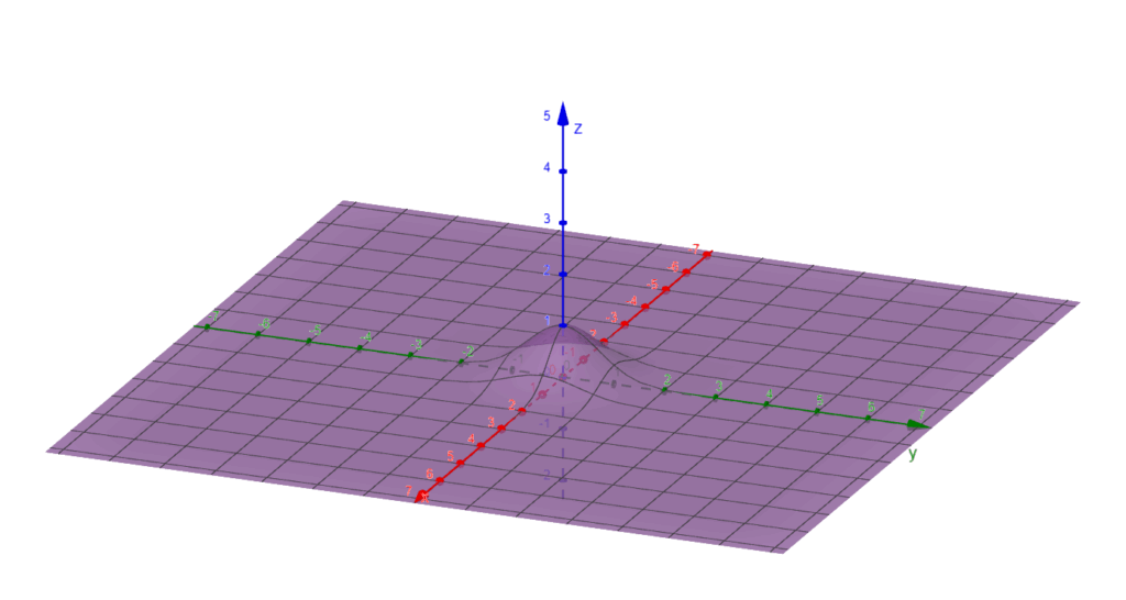
The surface of $f(x,y)=e^{-x^2-y^2}$. $f$ is maximal at the origin, where the gradient is zero.

Critical points play a crucial role in machine learning, especially when optimizing the loss function. The goal is to repeatedly update the parameters in order to minimize the loss.